Quickstart#
Install#
pip install hhgsfa
In a conda environment, activate it and run the same command. With uv, use uv add hhgsfa. The optional dependency
numba runs the SFA on every core, pip install "hhgsfa[numba]".
Units#
Everything is in SI units. Intensities are in W/m², so 1.5 × 10¹⁴ W/cm² is written 1.5e18. Both models use the
same time convention, \(e^{-i\omega t}\), so their phases can be compared directly. Fourier transforms are unitary.
Example#
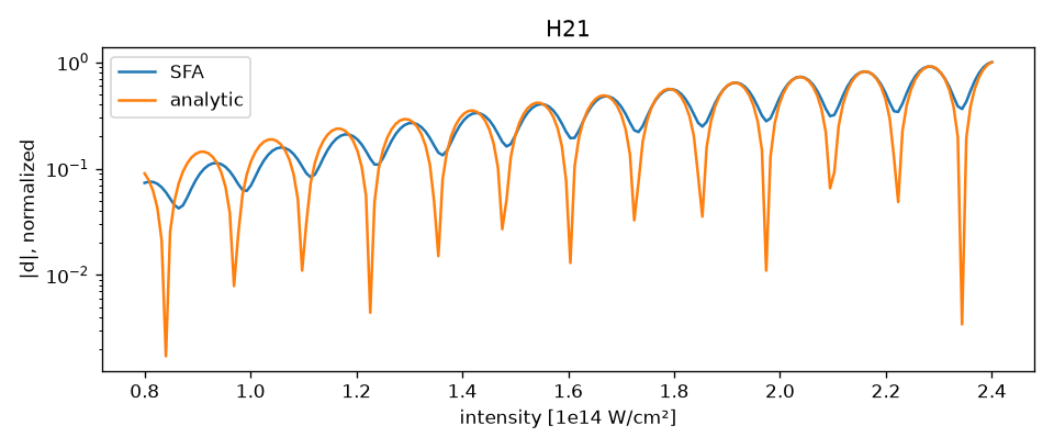
Harmonic 21 of a 1030 nm laser in argon, as the intensity grows. Both models show the same beating between the short and the long electron paths.
import matplotlib.pyplot as plt
import numpy as np

from hhgsfa import analytic, sfa

I = np.linspace(0.8e18, 2.4e18, 200)
d_sfa = sfa.harmonic_dipole(I, 21, "Ar", 1030e-9)
d_analytic = analytic.harmonic_dipole(I, 21, ("1", "2"), "Ar", 1030e-9)

fig, ax = plt.subplots()
for d, label in ((d_sfa, "SFA"), (d_analytic, "analytic")):
    ax.semilogy(I / 1e18, np.abs(d) / np.abs(d).max(), label=label)
ax.set(xlabel="intensity [1e14 W/cm²]", ylabel="|d|, normalized", title="H21")
ax.legend()
fig.tight_layout()
The user guide explains the two models.