Analytic model#
Each electron path gives the harmonic a phase that depends on the intensity. Guo et al. [1] showed that this phase follows a simple formula,
with coefficients \(a_j\) and \(b_j\) that depend only on the path \(j\) and the wavelength. They come from Guo et al. [1]
and Wikmark et al. [2], who call them \(\alpha\) and \(\gamma\). Here \(\alpha_j = \partial\phi_j/\partial I\) is the
slope of the phase, given by d_dipole_phase_dI.
path |
return |
\(c_a\) |
\(c_b\) |
\(c_{up}\) |
|
|---|---|---|---|---|---|
|
first |
short |
0 |
1.4 / 3.17 |
3.17 |
|
first |
long |
1 |
−1.2 / 3.17 |
3.17 |
|
second |
short |
1 |
1.0 / 1.54 |
1.54 |
|
second |
long |
1.4 |
−1.0 / 1.54 |
1.54 |
|
third |
short |
1.4 |
1.10 / 2.40 |
2.40 |
|
third |
long |
2 |
−1.10 / 2.40 |
2.40 |
with \(a_j = -c_a\,\alpha_\mathrm{fs}\lambda^3/(2\pi m_e c^3)\) and \(b_j = c_b\, m_e c/(2\alpha_\mathrm{fs}\lambda)\). A path only exists above its cutoff intensity, where \(q\hbar\omega = I_p + c_{up}U_p\), and the phase is NaN below it.
harmonic_dipole adds the paths you choose, \(d_q(I) = I^{q_\mathrm{eff}/2}\sum_j w_j e^{i\phi_j(I)}\), with the yield
growing as \(I^{q_\mathrm{eff}}\).
Example#
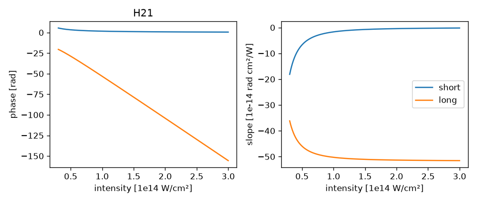
Harmonic 21 in argon at 1030 nm. The long path changes its phase much faster than the short one.
import matplotlib.pyplot as plt
import numpy as np

from hhgsfa import analytic

I = np.linspace(0.05e18, 3e18, 500)

fig, ax = plt.subplots(1, 2)
for path, label in (("1", "short"), ("2", "long")):
    ax[0].plot(I / 1e18, analytic.dipole_phase(I, 21, path, "Ar", 1030e-9), label=label)
    slope = analytic.d_dipole_phase_dI(I, 21, path, "Ar", 1030e-9) * 1e4 / 1e-14  # [1e-14 rad cm²/W]
    ax[1].plot(I / 1e18, slope, label=label)
ax[0].set(xlabel="intensity [1e14 W/cm²]", ylabel="phase [rad]", title="H21")
ax[1].set(xlabel="intensity [1e14 W/cm²]", ylabel="slope [1e-14 rad cm²/W]")
ax[1].legend()
fig.tight_layout()
References#
C. Guo et al., J. Phys. B 51, 034006 (2018).
H. Wikmark et al., PNAS 116, 4779 (2019).