SFA#
The SFA follows the electron after ionization, through the laser field and back to the ion, where it emits the harmonics. It is the model of Lewenstein et al. [1], with one electron, a linearly polarized field and no depletion of the ground state.
Functions#
function |
gives |
|---|---|
|
the dipole \(D(t)\) driven by any real field \(E(t)\) |
|
its spectrum |
|
its harmonic \(q\), exactly at \(q\omega\) |
|
the harmonic \(q\) at a fixed intensity |
The first three work on any pulse. harmonic_dipole answers a simpler question, what one atom emits at a given
intensity. It switches on a constant field, waits until the response repeats, and takes harmonic \(q\) over the last
cycle. That is the quantity of the analytic model.
Model#
In atomic units, with \(E\) the real field and \(A\) its vector potential,
The electron leaves at \(t - \tau\) and returns at \(t\), with momentum \(p_s = \frac{1}{\tau}\int_{t-\tau}^{t} A\,\mathrm{d}t'\) and action \(S = I_p\tau + \frac{1}{2}\int_{t-\tau}^{t} A^2\,\mathrm{d}t' - \frac{1}{2}\tau p_s^2\). The transition dipole \(d(p)\) is that of a hydrogen-like atom [2].
Numerics#
By default only the first return is kept, the short and long paths. Use
first_return=Falsefor every return.The time grid must resolve the cutoff, \(I_p + 3.17\,U_p\). A warning tells you how many points per cycle you need. About 128 per cycle is enough at 10¹⁴ W/cm² and 1 µm.
With numba installed, the calculation runs on every core. To use fewer, set the number of threads once, before the calculation.
import numba

numba.set_num_threads(4)  # hhgsfa then uses 4 cores
The same works from the shell, with NUMBA_NUM_THREADS=4 python script.py.
Examples#
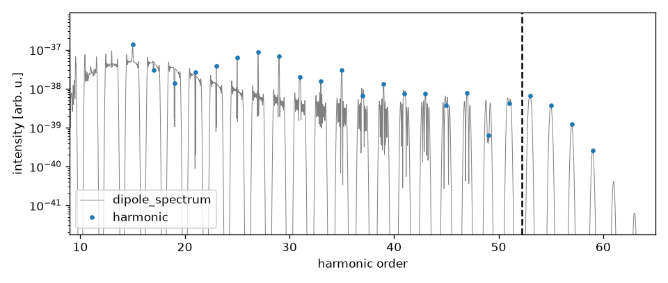
The spectrum of a 100 fs pulse at 1.5 × 10¹⁴ W/cm² in argon. The dots are harmonic on each odd order, and the
dashed line is the cutoff.
import matplotlib.pyplot as plt
import numpy as np
from scipy.constants import c, e, epsilon_0, h, m_e

from hhgsfa import sfa

wavelength, I0 = 1030e-9, 1.5e18
T = wavelength / c
t = np.arange(-220e-15, 220e-15, T / 128)
E = np.sqrt(2 * I0 / (c * epsilon_0)) * np.exp(-2 * np.log(2) * (t / 100e-15) ** 2) * np.cos(2 * np.pi * t / T)

D = sfa.dipole(t, E, "Ar", wavelength)
eV, S = sfa.dipole_spectrum(t, D)
q = np.arange(15, 60, 2)
H = sfa.harmonic(t, D, q, wavelength)

photon = h / T / e  # photon energy of the laser [eV]
Up = e**2 * I0 / (2 * epsilon_0 * c * m_e * (2 * np.pi / T) ** 2) / e  # ponderomotive energy [eV]
P = np.abs(S) ** 2
top = P[eV / photon > 9].max()
fig, ax = plt.subplots()
ax.semilogy(eV / photon, P, lw=0.6, color="0.5", label="dipole_spectrum")
ax.semilogy(q, np.abs(H) ** 2, "o", ms=3, label="harmonic")
ax.axvline((sfa.IP_AU["Ar"] * sfa.HARTREE_EV + 3.17 * Up) / photon, ls="--", color="k")
ax.set(xlim=(9, 65), ylim=(1e-5 * top, 5 * top), xlabel="harmonic order", ylabel="intensity [arb. u.]")
ax.legend(loc="lower left")
fig.tight_layout()
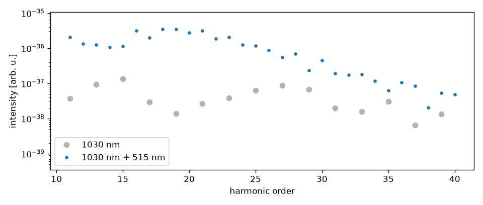
The same pulse with its second harmonic, 515 nm, added in phase at 10 % of the intensity. The field is no longer the
same from one half cycle to the next, so even harmonics appear. The dots are harmonic at every order.
import matplotlib.pyplot as plt
import numpy as np
from scipy.constants import c, epsilon_0

from hhgsfa import sfa

wavelength, I0 = 1030e-9, 1.5e18
T = wavelength / c
w = 2 * np.pi / T
t = np.arange(-220e-15, 220e-15, T / 256)  # the higher peak field needs more points per cycle
envelope = np.sqrt(2 * I0 / (c * epsilon_0)) * np.exp(-2 * np.log(2) * (t / 100e-15) ** 2)
q = np.arange(11, 41)

fig, ax = plt.subplots()
for E, label, style in (
    (envelope * np.cos(w * t), "1030 nm", dict(marker="o", ms=6, color="0.7")),
    (envelope * (np.cos(w * t) + np.sqrt(0.1) * np.cos(2 * w * t)), "1030 nm + 515 nm", dict(marker="o", ms=3)),
):
    H = sfa.harmonic(t, sfa.dipole(t, E, "Ar", wavelength), q, wavelength)
    ax.semilogy(q, np.abs(H) ** 2, ls="none", label=label, **style)
top = (np.abs(H) ** 2).max()
ax.set(ylim=(1e-4 * top, 3 * top), xlabel="harmonic order", ylabel="intensity [arb. u.]")
ax.legend(loc="lower left")
fig.tight_layout()
References#
M. Lewenstein, Ph. Balcou, M. Yu. Ivanov, A. L’Huillier and P. B. Corkum, Phys. Rev. A 49, 2117 (1994).
B. Podolsky and L. Pauling, Phys. Rev. 34, 109 (1929).